Decoding Messages in the Brain
Decoding the Language of the Brain
Welcome to my first blog post! My first few posts will be about the peer-reviewed publications that I have contributed to during my Masters and PhD thus far. Today’s blog is about my MSc thesis paper: Neural Burst Codes Disguised as Rate Codes, a title which will hopefully make sense by the end of this post!
The Big Picture (Background)
At a high level, the research question asked by my MSc paper is how can we understand the language of the brain?
The language of brain cells

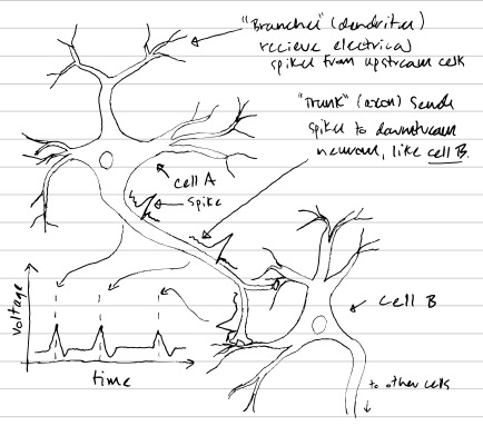
Your brain is composed of about 86 billion neurons–brain cells which are believed to be responsible for performing the computations that allow you to see, smell, think, talk, walk, and generally experience cognitive phenomena. To do this, these neurons communicate with each other, kind of like how a group of friends might text eachother to coordinate their work on a school project. However, while text chats are composed of words, neuron conversation is composed of electrical pulses that neuroscientists refer to as action potentials, or “spikes” (Fig.1).
Why we want to decode brain cell messages
Modern science doesn’t fully understand how to read the neural “spike language”. This is an important problem because if we could decode the spike-written messages between neurons, we would be one big step closer to understanding the brain, and could potentially solve medical problems–for example being able to control prosthetic devices just by thinking.
How neuroscientists think about brain cell messages

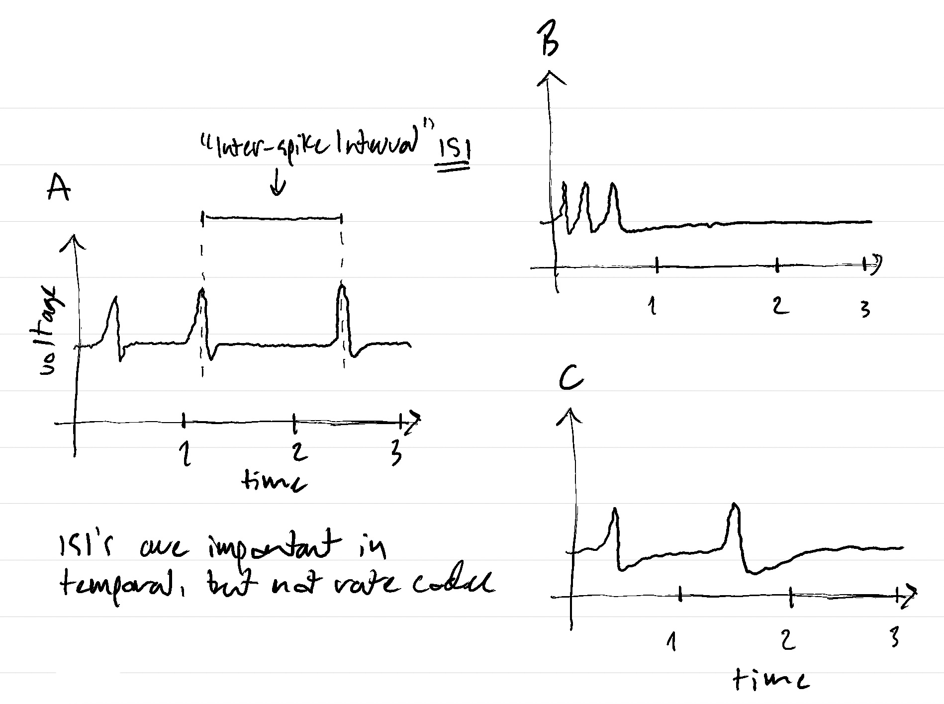
There are many theories for how to read the neural language, or “code”. These theories can be divided into two categories: rate codes and temporal codes. Rate code theories say that the only important aspect of the spike messages that a given neuron, neuron ‘A’, sends to another, neuron ‘B’, is the rate of spikes. If neuron A sends 1 spike every second for 3 seconds, then neuron B will see that neuron A’s spike rate is 1 spike per second. This will mean something different to neuron B than if A had sent 2 spikes per second during each of the three seconds–a spike rate of 2 spikes per second–but will have the same meaning as if neuron A had send 3 spikes to neuron B in the first second and no spikes in the next two seconds: 3 spikes in 3 seconds gives the same rate no matter which specific times within the three second window the spikes are sent.
Conversely, temporal coding theories say that the relative timing of the spikes does matter: that is, when neuron A sends 1 spike every second (Fig.2 A), this is different than if A had sent all 3 spikes in the first second (Fig.2 B). In this way, in a temporal code, when A sends 2 spikes separated by 1 second this would represent a different word than if A had sent B two spikes separated by
2 seconds\(^\dagger\).
My research paper looked at addressing a key question that appears in a certain class of temporal codes–how to resolve ambiguity between spike sequences.
Ambiguity in bursty brain cell messages

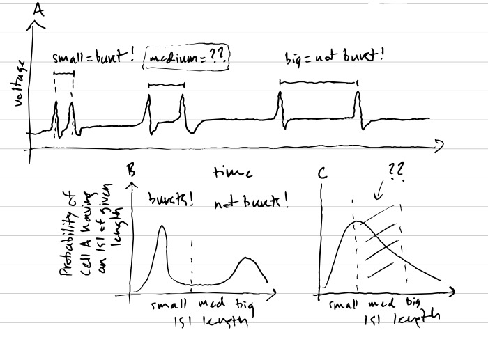
Imagine that you have a temporal code where spikes that occur really close together mean something different from spikes that occur farther apart. This kind of code is called a burst code because two or more spikes close together in time–bursts of spikes–mean something different than other, more spread out, spike sequences. Messages sent using this code will be easy to read if spikes only occur very far apart–making them clearly non-bursts–or very close together–making them clearly bursts. But what if they occur intermediate distances apart? If there is no hard threshold between what is considered a “burst” and what isn’t, then when neuron A sends neuron B spikes with time gaps of an intermediate length, there will be ambiguity when neuron B tries to understand what neuron A said because it won’t know if the spikes were a burst or not.
An analogy: imagine two friends, Bob and Alice, and that Bob is listening to Alice. Further imagine that Alice has a short attention span and is very rapidly switching back and forth between telling Bob about a performance of the nut cracker and explaining to Bob why almond milk is less sustainable than oat milk. To make it easier to tell when Alice is describing ballet or milk-alternatives, she talks about the former in french and the latter in english. However, there are many words that are the same between english and french, so when Alice says “festival”, it may not be clear to Bob whether this is a dance festival or a festival of flavours on the tongue brought on by a tasty milk alternative. These words that are the same in french and english are analogous to the spikes that are of intermediate distance apart, which we can’t immediately classify as bursts or non-bursts.
Importantly, experimental evidence shows that these ambiguous, intermediatly-spaced spikes occur frequently in the brain. It is thus an important question for neuroscientists whether neuron B can decode enough of the message from neuron A even with this ambiguity. If not, then neuroscientists will be able to scratch burst codes from the list of possible theories for reading the language of the brain.
What we did in my MSc Paper
Our specific research question was if neuron A can communicate effectively with neuron B even when there is ambiguity in whether a sequence of spikes can be considered a burst or not.
Our research methods
To answer this question, we needed a way of quantifying how well neuron B can decode neuron A’s spikes as a function of how much ambiguity there is in A’s spike messages. We took a computational approach to answer this question, meaning that we came up with a mathematical model of neurons A and B–a set of equations describing the spikes that A produces and the machinery that B uses to decode those spikes–and analyzed a computer simulation of this model. In this model, we could vary the amount of ambiguity in A’s messages. We then used tools from information theory to quantify how well model neuron B could decode model neuron A’s messages. Information theory is a branch of mathematical statistics that quantifies the amount of predictability (vs unpredictability, or ambiguity) in a variable object. In particular, information theory can also be used to evaluate how predictive one variable is of another. For example, one pair of variables could be (1) the identity of a card in a deck (e.g. ace of spades) and (2) the colour of the card. The information contained in card colour about the identity of the card is not super high (e.g. there are many, 26, cards in a deck that are red). If variable (2) was instead card number/face this would be comparatively more predictive (e.g. there are only 4 kings in a deck, narrowing the options). In our case, variable (1) would be a time-varying signal encoded in the bursty spikes of model neuron A, and variable (2) would be the read-out taken by model neuron B.
Our findings and why they are useful
We found that, in certain cases, neuron A can communicate quite effectively with neuron B, even when there is ambiguity between which spike pairs should be considered bursts and which should be considered non-bursts! Interestingly, in such cases, the statistics of neuron A’s spiking look very similar to how they would look if neuron A was using a rate code. This means that if an experimentalist records neuron activity in the brain and finds that a neuron’s spiking looks like a rate code it might actually be stealthily using a temporal, bursting code! Hence the name of the paper.
For a brief overview of some of the math used, and for some key references, see below. Thanks for reading!
Math Overview
Neural Circuit Model
I’m not including the equations in this section as they are bulky and don’t provide too much intution. See the supp of our paper for them.
- For neuron A, we formulated a new bursting model, the Burst Spike Response Model, inspired by the Spike Response Model of Gerstner et al and previous work by my MSc supervisor Richard Naud. Mathematically, the model is a point process determined by an event rate and a burst probability: the former determines how often spikes occur and the latter determines whether or not a rapidly-occurring burst spike occurs after the original spike. In neuro-theory language, this is a two compartment model with stochastic spiking, where the first (dendritic) compartment encodes the burst probability and the second somatic compartment encodes the event rate
- The inputs to neuron A are Ornstein-Uhlenbeck processes
- Neuron B is modelled as a nonlinear function of the linearly filtered spike train of neuron A
Info Theory Analysis
To quantify information transmitted we used the mutual information rate, \(\mathbb{I}\), a generalization of mutual information from random variables to stochastic processes:
\[\mathbb{I}(X, Y) = \lim_{T \to \infty}\frac{1}{T}I(X_{0:T};Y_{0:T}),\]where \(X\) and \(Y\) are stochastic processes and \(I(X_{0:T};Y_{0:T})\) is the mutual information between the vector \(X_{0:T} = [X_0, ..., X_T]\) and \(Y_{0:T} = [Y_0, ..., Y_T]\).
This quantity is a massive hassle to compute, but one can compute a linear lower-bound for this information rate as:
\[-\int_0^{\frac{1}{2}}\log_2\big(1 - \Phi_{XY}(f)\big)\mathrm{d}f,\]where \(\Phi_{XY}(f)\) is the coherence between \(X\) and \(Y\) and \(f\) is frequency (see Stein et al.). We used this to quantify information transmitted in the paper. The fact that we only quantified the linearly encoded mutual information rate, rather than taking into account all (potentially nonlinearly encoded) information, is a shortcoming of this work and something that could be explored in future research!
References
For further reading on a given topic, see below (papers are author first; textbooks are title first):
- Neural coding:
- Burst coding
- Modelling neurons
- Information theory
- Information theory applied to neuroscience
- Neural Burst Codes Disguised as Rate Codes
In-blog footnotes
- \(\dagger\) : one may notice that the difference between rate and temporal codes is a little more subtle than described above. One could imagine a situation where the stimulus being encoded in the firing rate of cell ‘A’ changes very quickly, and the downstream cell decoding A’s message is very sensitive to each spike. In this case, even with a rate code small differences in spike timing could convey information. In this way, the real distinction between rate and temporal codes depends on whether there is information in cell A’s spike train at higher frequencies than those of the stimulus that cell A is encoding. See the Theunissen & Miller ref for more details.